Notebook Usage

Open Dashboard, create Python3 Notebook by selecting New - Python3, will then enter Python3 Notebook interactive programming environment. At the same time, an IPython Notebook file named untitled.ipynb is generated for this interaction.

This section will introduce a basic Hello World, a Visualizing Machine learning result, a complete tutorial.

Hello World

In a new Cell, input Python3 code:

print("Hello World")

Run and get the result:

Hello World

Visualizing Machine Learning Result

Visualizing need the support of matplotlib. It should be loaded first.

Input and execute the following code in a new Cell:

%matplotlib inline

or

%matplotlib notebook

If no error, the browser is now ready to draw graphs.

Input and execute the sample machine learnign code in a new Cell:

# import package
import numpy as np
import matplotlib.pyplot as plt
from sklearn import linear_model, datasets

# load data : we only use target==0 and target==1 (2 types classify) and feature 0 and feature 2 ()
iris = datasets.load_iris()
X = iris.data[iris.target!=2][:, [0,2]]  
Y = iris.target[iris.target!=2]

h = .02  # step size in the mesh

logreg = linear_model.LogisticRegression(C=1e5)
logreg.fit(X, Y)

# Plot the decision boundary. For that, we will assign a color to each
# point in the mesh [x_min, m_max]x[y_min, y_max].
x_min, x_max = X[:, 0].min() - .5, X[:, 0].max() + .5
y_min, y_max = X[:, 1].min() - .5, X[:, 1].max() + .5
xx, yy = np.meshgrid(np.arange(x_min, x_max, h), np.arange(y_min, y_max, h))
Z = logreg.predict(np.c_[xx.ravel(), yy.ravel()])

# Put the result into a color plot
Z = Z.reshape(xx.shape)
#plt.figure(1, figsize=(4, 3))
plt.pcolormesh(xx, yy, Z, cmap=plt.cm.Paired)
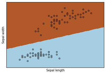
plt.xlabel('Sepal length')
plt.ylabel('Sepal width')

# Plot also the training points
plt.scatter(X[:, 0], X[:, 1], c=Y, edgecolors='k', cmap=plt.cm.Paired)
plt.xlabel('Sepal length')
plt.ylabel('Sepal width')

plt.xlim(xx.min(), xx.max())
plt.ylim(yy.min(), yy.max())
plt.xticks(())
plt.yticks(())

plt.savefig("learn.svg")

Later on, you will see the output like:

At the same time, a vector graph learn.svg is generated in the current directory, which can be opened in the Dashboard.

You can also open it directly here by input and execute

SVG("learn.svg")

Complete Tutorial

Many tasks can be done in IPython Notebook, some are interesting, for example, displaying kinds of JPG/PNG/SVG pictures, videos, HTML files, pdf files, loading external resources like an remote WEB page, even a Youtube video, showing LaTeX math formula, etc.

The complete user guide and tutorials can be refered here.

Jupyter nbviewer also shows many examples.