使用 Notebook

进入 Dashboard , 选择 New - Python3, 创建 Python3 Notebook, 会 进入 Python3 Notebook 交互编程环境，并生成一个 untitled.ipynb 的 IPython Notebook文件。

本节介绍了一个基本的Hello World, 一个机器学习并可视化结 果, 一个完整教程 的链接。

Hello World

在 Cell 中输入

print("Hello World")

执行后得到输出

Hello World

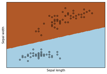
一个机器学习并可视化结果的示例

绘图需要加载 matplotlib. 在 Cell 中输入并执行

%matplotlib inline

或者

%matplotlib notebook

即可开启在浏览器中绘图的支持。

在后面的 Cell 中输入并执行下面关于机器学习的代码

# import package
import numpy as np
import matplotlib.pyplot as plt
from sklearn import linear_model, datasets

# load data : we only use target==0 and target==1 (2 types classify) and feature 0 and feature 2 ()
iris = datasets.load_iris()
X = iris.data[iris.target!=2][:, [0,2]]  
Y = iris.target[iris.target!=2]

h = .02  # step size in the mesh

logreg = linear_model.LogisticRegression(C=1e5)
logreg.fit(X, Y)

# Plot the decision boundary. For that, we will assign a color to each
# point in the mesh [x_min, m_max]x[y_min, y_max].
x_min, x_max = X[:, 0].min() - .5, X[:, 0].max() + .5
y_min, y_max = X[:, 1].min() - .5, X[:, 1].max() + .5
xx, yy = np.meshgrid(np.arange(x_min, x_max, h), np.arange(y_min, y_max, h))
Z = logreg.predict(np.c_[xx.ravel(), yy.ravel()])

# Put the result into a color plot
Z = Z.reshape(xx.shape)
#plt.figure(1, figsize=(4, 3))
plt.pcolormesh(xx, yy, Z, cmap=plt.cm.Paired)
plt.xlabel('Sepal length')
plt.ylabel('Sepal width')

# Plot also the training points
plt.scatter(X[:, 0], X[:, 1], c=Y, edgecolors='k', cmap=plt.cm.Paired)
plt.xlabel('Sepal length')
plt.ylabel('Sepal width')

plt.xlim(xx.min(), xx.max())
plt.ylim(yy.min(), yy.max())
plt.xticks(())
plt.yticks(())

plt.savefig("learn.svg")

稍后可看到如下输出

当前目录下同时会生成矢量图形文件 learn.svg，可以在 Dashboard 中打 开， 也可以直接在 Cell 中打开

SVG("learn.svg")

完整教程

在IPython Notebook中 能做很多事情，如显示本地磁盘中的各种图形文件、视频 文件、HTML文件，加载一个外部网站，显示 LaTeX 公式等，完整介绍和教程请见 这里.

nbviewer 同样提供了很多其他应用示例。